
An accessible guide to dispersion modelling and AI prediction with practical applications.
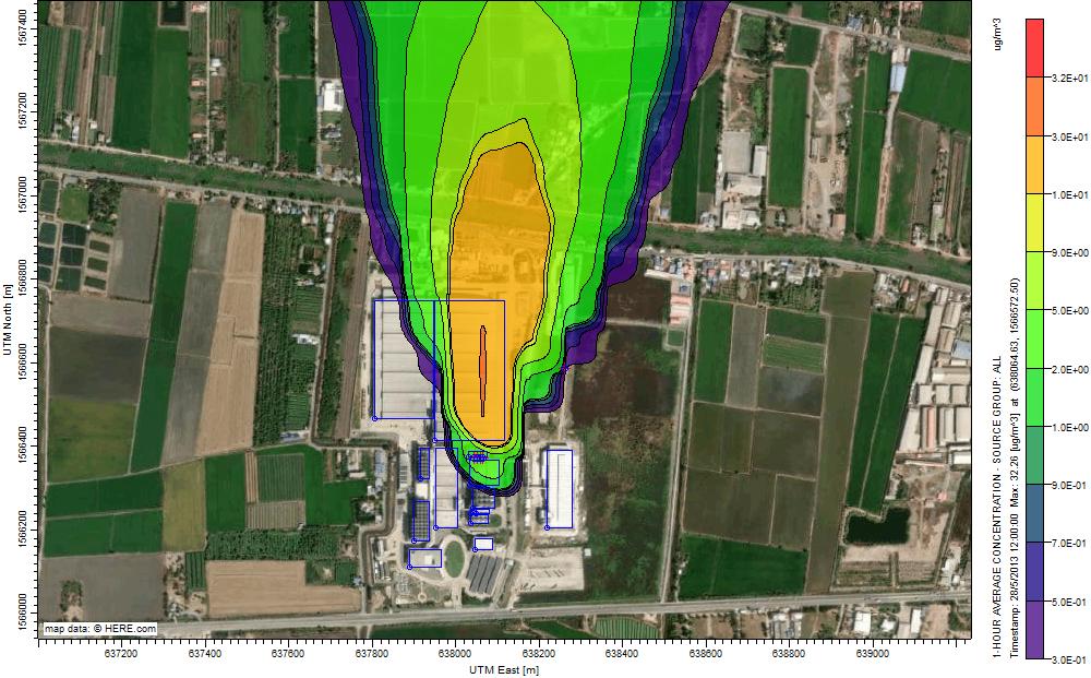
A regulatory dispersion model answers one kind of question: over a full year, what is the highest concentration at the receptors, and does it exceed the standard? That answer comes from running a full year of meteorological data and takes hours to days of computation.
The question that actually arises on site is different: it is 14:20 — where is the odour the community is complaining about coming from, and where will it go in the next two hours? Real-time dispersion systems exist to answer the second kind of question. This article explains what such a system is made of, how it computes fast enough to be useful, where AI genuinely helps, and what to verify before trusting the output.
Regulatory versus real-time modelling
Both use the same physics but differ in purpose, inputs, and time constraints. Confusing the two — using the output of one where the other is required — is the most common mistake in practice.
| Aspect | Regulatory model | Real-time model |
|---|---|---|
| Question answered | Does the annual maximum exceed the standard? | Where is the plume now and over the next few hours? |
| Meteorological input | 1–5 years of historical data processed through AERMET | Local station data in real time plus numerical weather prediction |
| Averaging period | 1-hour to annual | 1–15 minutes |
| Direction of computation | Forward, source to receptor | Both forward and backward, receptor to source |
| Acceptable runtime | Hours to days | Seconds to minutes |
| Typical output | Maximum concentration tables and isopleth maps | Animated maps, alerts, and ranked source likelihoods |
| Legal standing | Citable in permit applications and impact reports | A management tool; does not replace statutory measurement |
A five-layer system architecture
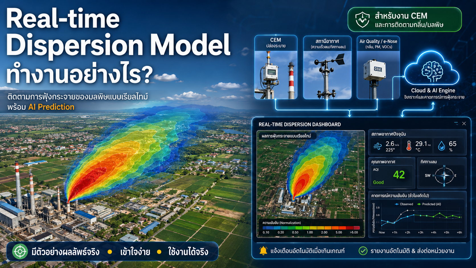
- Input layer: source emission rates from continuous emission monitoring systems (CEMS) at main stacks, or estimates from operating logs for sources without installed instruments; fenceline ambient measurements of indicator gases such as H2S, NH3 and total VOCs, particulate matter, and sensor arrays used for odour monitoring; on-site meteorological data—including wind direction and speed at the reference height, temperature, humidity, solar radiation, and variables used to assess atmospheric stability—from a local station rather than one tens of kilometres away; numerical weather forecasts for 6–48-hour outlooks; and operating and complaint logs that turn attractive maps into evidence that can be explained and defended.
- Data quality layer: range, spike and flatline tests, drift detection, and collocation-based correction. This layer determines how many false alarms the system produces and is the one most often neglected. Machine-learning correction trained against reference instruments is well supported for low-cost sensor networks, provided the correction is reviewed periodically. [5]
- Dispersion engine: selected according to the required response time and spatial scale, as explained in the next section.
- Analysis layer: forward calculation to estimate concentrations at receptors from known emission rates; backward calculation to identify the sources most likely to explain measured values; anomaly detection by comparing measurements with modelled expectations, where a large discrepancy may indicate an unlisted source; and time-specific risk ranking based on wind direction, distance, and sensitive receptor locations.
- Alerting and visualisation layer: every alert must be tied to a predefined action: at watch level, inspect the treatment system; at warning level, slow down activities with high odour emissions; and at critical level, temporarily suspend the activity and notify management. Without predefined actions, alerts become background noise within weeks.
The data quality layer deserves particular attention. A real-time model cannot produce a reliable answer from unreliable measurements, regardless of the sophistication of its computation engine.
| Check | What it detects | Response |
|---|---|---|
| Range check | Physically impossible values, such as negative concentrations | Reject the value and flag it as invalid |
| Spike test | Electrical noise or highly localised interference | Compare with neighbouring sensors before deciding |
| Flatline test | A frozen sensor or disconnected signal cable | Issue a maintenance alert, not a pollution alert |
| Drift check | A sensor baseline that shifts as the instrument ages | Recalibrate or correct the reading with a calibration model |
| Collocation calibration | Error relative to a reference instrument | Develop a correction equation and review it periodically |
Choosing a computation engine
The binding constraint in real-time work is time, not physical fidelity. The most accurate methods are usually too slow to inform a decision.
| Method | Principle | Approximate runtime | Best suited to | Key limitation |
|---|---|---|---|---|
| Short-averaging Gaussian plume | Steady-state analytical solution recomputed each short interval | Seconds | Known point sources, simple terrain | Breaks down in calm or rapidly veering winds |
| Lagrangian puff (CALPUFF, SCIPUFF) | Release represented as puffs advected by a time-varying wind field | Seconds to minutes | Calm and variable winds, medium to long range | Requires a good three-dimensional wind field |
| Lagrangian particle (HYSPLIT, FLEXPART) | Tracks large numbers of virtual particles | Minutes | Long range, backward runs, wildfire smoke and volcanic ash [3] | Requires continuous gridded meteorology |
| CFD | Solves the flow around buildings and obstacles directly | Hours to days | Congested sites where buildings govern the flow | Too slow for direct real-time use |
| Pre-computed response fields | Unit-emission concentration fields computed offline for a matrix of conditions, then scaled at runtime | Sub-second | High update rates with fixed sources | Covers only the pre-computed conditions |
| Machine-learning surrogate | A model trained to reproduce CFD or physics-model output | Sub-second | Bringing CFD-level detail into fast applications [4] | Reliable only inside the training envelope |
The practical trick that makes real-time operation possible is the linearity of the dispersion equation: concentration scales directly with the emission rate Q, and contributions from multiple sources superimpose. [1] Unit-emission fields can therefore be computed offline for, say, 36 wind directions × 6 wind speed bins × 6 stability classes, then simply selected and scaled at runtime. The underlying physics remains the standard model.
Backward calculation: from measurement to source
| Approach | Requires | Produces | Best for |
|---|---|---|---|
| Directional statistics (bivariate polar plots, conditional bivariate probability function) | Months of paired concentration and wind data | The wind directions and speed ranges associated with high readings, pointing to source location [6] | Low-cost, repeatable initial screening |
| Reverse plume modelling | Candidate source locations and contemporaneous wind data | The emission rate required to produce the measured concentration [7] | Cases where the candidate sources are known |
| Source term estimation by optimisation | Multiple receptors and a good wind field | The location and emission rate that best explain all receptors simultaneously | Releases of unknown origin |
The inverse problem is ill-posed: a distant strong source and a nearby weak one can produce identical readings at a single receptor. Results should therefore be reported as ranked likelihoods with uncertainty, not as a single definitive answer, and at least three receptors distributed around the area are needed to separate sources that lie along the same bearing.
What AI can and cannot do
The term AI is used very broadly in the market. It is therefore important to identify exactly where the algorithm contributes before making an investment decision.
| Task | Role of the algorithm | Confidence |
|---|---|---|
| Sensor correction and drift compensation | Regression or machine learning against collocated reference data | High, well supported by literature [5] |
| Computational acceleration | Surrogate models trained on physics-model output | High within the training envelope [4] |
| Anomaly detection | Comparison of measured against expected behaviour | Medium to high |
| Odour signature classification | Pattern recognition on sensor arrays | Medium; depends chiefly on the training set |
| Predicting concentration without physics | Purely data-driven models | Low outside the conditions seen in training |
Three limitations belong in every proposal. Data-driven models cannot reliably predict conditions absent from their training data, such as a large release that has never occurred before. Emission rate uncertainty is the dominant source of error in this field, and no algorithm compensates for wrong inputs. And real-time output is a calculated value, not a statutory measurement — it must be labelled as such every time it is presented.
Example of an operational timeline
The following example shows the sequence from detection to confirmation and illustrates what “real time” means in practice.
| Time | Event | System response |
|---|---|---|
| 13:55 | The eastern fenceline station records a threefold increase in an indicator gas within ten minutes. | The data are logged and passed to the quality-control layer. |
| 13:56 | The reading is checked against neighbouring stations to confirm that it is not a noise spike. | The event is confirmed as genuine. |
| 13:57 | A backward calculation is run using the wind data at that time. | Possible sources are ranked with confidence values. |
| 13:58 | The system issues an alert with the predicted plume direction for the next two hours. | The operator receives a message and a map. |
| 14:05 | The site is inspected according to the predefined response procedure. | The cause is found and corrective action is taken. |
| 14:30 | The station readings return to their normal level. | The system closes the event and stores it as a case record for future reference. |
The real value lies not merely in the alert but in the complete event record. If a complaint is received later, the facility can show when the event occurred, how long it lasted, where the wind was blowing, and how many minutes it took to take corrective action. That is a very different level of evidence from simply stating that the facility was under control.
Assessing system reliability
Before using the output for decisions, performance should be assessed in two separate dimensions: model accuracy against measurements and the operational quality of the alerts.
| Metric | Meaning | Reference guidance |
|---|---|---|
| FAC2 | Fraction of predictions within a factor of two of observations | Higher is better; roughly 50% or more is commonly expected in simple conditions [2] |
| Fractional bias (FB) | Systematic over- or under-prediction | Low absolute value; a mean bias below roughly 30% is generally regarded as good [2] |
| NMSE | Combined systematic and random error | Lower is better |
| False alarm rate | Share of alerts with no verified cause | Agree a target with operators; too high and the system is ignored |
| Missed detection rate | Share of real events not alerted | More important than false alarms in safety applications |
| Lead time | Interval between alert and receptor impact | Longer lead time is the whole value of prevention |
The first group follows the model evaluation framework of Chang and Hanna (2004), which stresses that acceptable performance depends on scenario complexity, source term uncertainty, and meteorological data quality — so a single threshold should not be applied to every case. [2]
Limitations to state explicitly
- Calm winds: steady-state plume models lose physical meaning as wind speed approaches zero, which is precisely when night-time odour complaints occur. Puff or particle models are required instead. [1]
- Emission rate uncertainty dominates the error budget, and area and intermittent sources are usually unmeasured.
- Meteorological representativeness: wind data from a distant station in different terrain can put the modelled plume in the wrong direction entirely.
- Sensor drift requires a documented calibration schedule, without which the record cannot be used retrospectively.
- Legal standing: real-time output supports management decisions; statutory proof still requires the measurement methods prescribed in the applicable regulation.
Key takeaways
- Real-time and regulatory models answer different questions and are not interchangeable.
- Speed comes from computational design, such as pre-computed unit-emission fields, not from weakening the physics.
- Backward calculation yields ranked possibilities, not a single answer, and needs multiple receptors.
- AI is clearly useful for calibration, acceleration and anomaly detection, but does not substitute for correct inputs.
- Evaluate both model accuracy and alert quality, or the system will be ignored within months.
Consult an expert
RE-VEAL designs and installs continuous air-quality and odour monitoring systems integrated with dispersion models for surveillance and alerting. The service covers station siting, data quality control, integration with local meteorological data, and retrospective reporting for complaint response. Contact our team to assess the suitability of the system for your site.
References
- Stockie, J. M. (2011). The Mathematics of Atmospheric Dispersion Modelling. SIAM Review, 53(2), 349–372.
- Chang, J. C., & Hanna, S. R. (2004). Air quality model performance evaluation. Meteorology and Atmospheric Physics, 87, 167–196.
- Stein, A. F., et al. (2015). NOAA’s HYSPLIT Atmospheric Transport and Dispersion Modeling System. Bulletin of the American Meteorological Society, 96(12), 2059–2077.
- Hazardous atmospheric dispersion in urban areas: A deep learning approach for emergency pollution forecast (2022). Environmental Modelling & Software.
- Zimmerman, N., et al. (2018). A machine learning calibration model using random forests to improve sensor performance for lower-cost air quality monitoring. Atmospheric Measurement Techniques, 11(1), 291–313.
- Uria-Tellaetxe, I., & Carslaw, D. C. (2014). Conditional bivariate probability function for source identification. Environmental Modelling & Software, 59, 1–9.
- Developing an odour emission factor for an oil refinery plant using reverse dispersion modeling (2019). Atmospheric Environment, 218.
- U.S. Environmental Protection Agency. Guideline on Air Quality Models, 40 CFR Part 51, Appendix W (as revised, 2024).